General Architecture

First we applied a dimensionality reduction scheme converting each input vector (originally of dimension 242 and 352) into a low-dimension vector consisting of a mixture of two types of coordinates - distances from a given number of cluster centers, and choosing highest-entropy coordinates from the original data.

Next,  an ensemble of three types of RBF networks was optimized. We have used Bishop's netlab code and two types of Orr's RBF code. Each net was optimized according to relevant input parameters, and a confidence estimate was retained. The confidence was based on a cross validation scheme.

Networks of the same type in the ensemble differed by two criteria: They were trained on different random subsets of input vectors, and the optimization procedure had a random element in it.

Then, a reconstruction constraint was added to the networks, and a supervised gradient descent learning process on all the parameters of the network was performed. The nets were again estimated for confidence, and in case of improvement the old net was replaced by the new net in the ensemble.

Finally one of 4 ensemble fusing methods can be chosen to use the ensemble as a classifier for new data.

Source Code Usage

Click here to obtain a zip file with bug-fixed Bishop netlab code

Click here to obtain a zip file with Orr's code (Note that Orr's code is zipped in subdirectories. Make sure your matlab path points to subdir "meth" and "util")

Click here to download this HTML document with images(zipped)

Source code consists of three functions and some helper functions, in addition to Orr's and Bishop's code. Some bugs in Bishop's code have been fixed, and therefore it is vital to use this version of NETLAB.

Below are the options of the main functions.
 

[processed, preproc] = findpreproc(train_data, train_label, procoptsions, preproc)

Requirements: This function has two tasks. First it finds an optimal preprocessing and second, it generates the pre-processed data. If preproc is supplied, the program runs the data through the preprocessing methodology which should be completely kept in preproc.

Usage:
 

Depending on the number of arguments:    3 - find an optimal preprocessing for a given training data    4 - runs the data through the preprocessing method. Doesn't need        the T input in this mode.    X - training data,    T - target values (can be empty when preproc is supplied)    OPTIONS (1) - data set: 0 - 'sonl' or 1 - 'psd'    OPTIONS (3) - number of entropy coordinates to choose or 0 for optimal value    OPTIONS (4) - number of cluster centers to use or 0 for optimal value    OPTIONS (5) - nonzero: use gaussian kernel estimation in entropy evaluation                 (more precise, but time consuming)    OPTIONS (6) - nonzero: use mahanalobis distance in clustering                  (very very time consuming)    ---   Uses "rentropy" code from previous year written by Faran, Mertens and Keinan

[preproc, netarch] = findarch(train_data, train_label, options)

Requirements: This function finds an optimal preprocessing and a set of architectures with their corresponding parameters which are best for the given training data. This function calls internally to findpreproc.

Usage:
 

OPTIONS(1) to (6) are for the preprocessing:      OPTIONS (1) - data type: 0 - 'sonl' or 1 - 'psd'    OPTIONS (3) - number of entropy coordinates to choose or -1 for optimal value    OPTIONS (4) - number of cluster centers to use or -1 for optimal value      OPTIONS (5) - nonzero: use gaussian kernel estimation in entropy evaluation                 (more precise, but time consuming)      OPTIONS (6) - nonzero: use mahanalobis distance in clustering                  (very very time consuming)        The other options are for the network training      OPTIONS (7) - number of networks for each architecture in the ensemble                  default = 6     OPTIONS (8) - size of sample from data for each net (default 55)    OPTIONS (9) - lamda - relative part of reconstruction constraint in error (default 0.1)    OPTIONS (10) - type of ensemble fusing:                      0 - weighted voting                     1 - simple voting                     2 - weighted mean                     3 - simple mean      uses 'check_bias' code from last year written by Helman, Zivan and Friedrich

[label_pred, confidence] = netpred(data, preproc, netarch, options)

Requirements:  This function performs the preprocessing on the given data based on the preprocessing scheme that was chosen by findarch and is stored in preproc and then prediction of the  class labels based on the architectures that were found by findarch and are stored in  netarch. Note that if a collection of several experts is found by findarch, then the algorithm for fusing the experts should also be stored in netarch to be used by netpred.  You should suggest a way to calculate the confidence and justify in your written report why this confidence method is useful.

Usage:
 

CONFIDENCE is a structure containing fields:        VAR - variance of classification results       DIST - distance of raw classification from 0.5    [pred, confidence, y] = netpred (X, preproc, netarch, options)        returns also raw classifications from each classifier    OPTIONS(1) and (6) are for the preprocessing:    OPTIONS (1) - data type: 0 - 'sonl' or 1 - 'psd'    OPTIONS (6) - nonzero: use mahanalobis distance in clustering preprocessing                  (very very time consuming)

Preprocessing

preprocessed = [ prep_cluster  prep_entropy ];
 

Clustering

Source code:

• find_clusters.m - find cluster centers and cov-matrix
• prep_clusters.m - calculate distance from cluster centers

• An initial clustering is performed using klogk clusters, and then the actual clustering is done.
• Mahalanobis distance weighs heavily on performance, and didn't seem to improve later classification results.
• Due to sparse input data. when calculating mahalanobis distance, there can be a one-sample cluster, which disallows standard computation of the mahalanobis distance. A pseudo-inverse of the covariance matrix was used to overcome this problem.
• In general, we have not succeeded in finding a consistently optimal number of cluster centers. Clustering data did not, usually lead to good classification, and finally, a low number of cluster centers (3-5) was chosen as a default for our implementation.

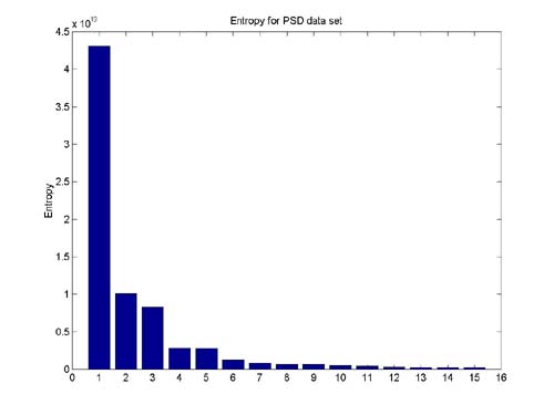
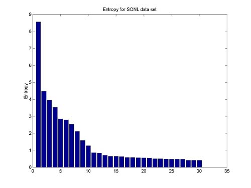
Maximal Entropy

Source code:

rentropy.m - from last year's class (with bug fixes)

• Looking at a visualization of the entropy values (below) across the coordinates, one can see very clearly the variance between the different dimensions' entropy in each one of the data sets. These graphs have been used by us as a starting point for the optimization of the default values for number of high-entropy coordinates.
• An automated procedure can be considered, cutting entropy coordinates according to first order derivative of the below graph. We have tried such a procedure on the given data sets with great success. The cutting point is then decided by defining a threshold for entropy derivative normalized by the entropy value. More data sets should be examined to determine general properties of this method.
• Entropy based coordinates have proved a good preprocessing method in subsequent classification tasks.

Normalization

Another normalization was performed on the combined output of the two preprocessing methods to prevent extreme influence of certain coordinates on optimization and learning.

Source code:

normalize.m

RBF Net Optimization

Source code:

optimal_net.m - Finding optimal network parameters for each of the types

RBF by Bishop

Source code:

optimize_bishop.m

• During hidden layer construction (the EM algorithm) we discovered that there are cases of zero values in the probability matrix. Since this caused division by zero error, we took a precautionary measure and added epsilon to this matrix (see gmmem.m).
• We have not found an optimal number of hidden units, but due to the random nature of the basic network training, a good network is usually found at one of the range of hidden unit numbers.
• In very broad terms, more hidden units result in better classification, but it is not a monotonous relationship.
• More hidden units do, of course, hold the danger of overfitting the specific data.

RBF by Orr

Orr does an automatic selection of the number of hidden units. Three important parameters can, though, be optimized:

Constant radii

The initial RBF radii can either be relative to the spread of the input data on each coordinate, or equal sized along the coordinates.

Scale of widths

RBF radii can be initialized with a multiplier called "scale", to enrich the mixture of the RB functions.

Bias

A boolean modifier to specify whether to use a bias unit in the second layer or not.

We performed optimization on the scales in an iterative way (with the help of previous year work) and found that for the "forward selection" scheme it is best to optimize the scales between [0.75 1 1.25], whereas for the "ridge regression" scheme an open optimization is benefitial. In addition, the usage of constant radii and bias is used only on the "ridge resgreesion" scheme (according to experimental results).

Remarks:

• In general, we have found Orr's networks to tend to overfit the input data, since a large number of RBF centers is usually selected in the optimization algorithms applied by Orr. This results in a misleading cross validation error measure, which is usually lower than its generalization value (and negatively influences the ensemble fusing).
• We have found constant radii to work better with the SONL data and worse with the PSD data. This conclusion should be further verified with more data.

Reconstruction Constraint

The networks from the optimization step were added the reconstruction constraint in the form of additional output targets, and then a gradient descent optimization on the RBF parameters was performed according to the formulae below:

The error function that was optimized was a weighted combination of the y- target and the reconstruction target (divided by the size of the reconstruction vector). This weighting is governed by the lamda parameter, that the user can modify (default 0.1).

Source code:

• add_reconstruction.m
• remove_reconstruction.m
• netopt_recons.m

• For good (low error) networks from the first stage, the reconstruction stage rarely yielded an improvement over the training data. If the first stage optimization of a network in the ensemble was less successful in classifying the test data, reconstruction usually improved the error value slightly.
• The reconstruction optimization does not converge if the number of parameters (i.e. hidden units) is too large. Therefore, on most of the networks from Orr's code the reconstruction step did not succeed to lower the error.
• If a low number of hidden units is selected in Bishop's code, then the reconstruction step is usually effective.
• In choosing the number of optimization iterations, there is a tradeoff between the computation time and the quality of the improvement.

Ensemble Fusing

1. Weighted Voting (default) - Each network votes on the classification (0 or 1) and each vote has a relative weight according to the network's confidence.
2. Simple Voting  - Each network votes on the classification (0 or 1) and each vote has the same weight regardless of the network's confidence.
3. Weighted Mean - The prediction is based on the mean of the networks' output. Each output has a relative weight according to the networks confidence.
4. Simple Mean - The prediction is based on the mean of the networks' output.

• Even though the weighting vote was found to be the best predictor, there still remains a problem of filtering bad networks that got a good error-confidence in the first stage. We have found several networks that passed the first confidence stage with very good results, and had a very poor prediction value. This had a negative influence on the overall prediction.

Ensemble Confidence

1. Variance - Low variance of prediction between networks implies a good ensemble confidence.
2. Significance - Another method of computing the confidence of the prediction is the output's distance from 0.5, which is basically a computation of the significance of the prediction.

Conclusions

In addition, the reconstruction constraint has a positive effect only on initially badly performing networks, and many times, even though the reconstruction abilities of the network improved, the classification abilities didn't improve, and sometimes even deteriorated.

As to the data sets, the SONL data set is much easier to classify, and the entropy preprocessing stage implies that many of the PSD coordinates are too low-entropy to give any good indication as to the nature of the data. Finally, we couldn't achieve very good results on the PSD set, whereas for the SONL set an almost-perfect classification was often found.

In the preprocessing stage, the number of entropy based coordinates have proven to be crucial to the success of the classification. Too little, but also too many, coordinates worsen the classification immensely. The clustering preprocessing was found to be less than optimal.

Two types of error were used in the cross validation stage: The error over all the data (train and test), and error on the test data alone. The latter seems to characterize the generalization traits of the network better.

The expert fusion was not investigated enough, but initial results point to the "weighted vote" option as being optimal. Some problems remain, though, especially with "fake experts", i.e. nets that performed well on the optimization step, but don't generalize well over new data. This is a problem especially with Orr's networks.
 

Future Work

• A minimal entropy constraint on the first layer parameters has yet to be implemented.
• Find better optimization for the PSD data set.