Submitted by:

Igor Bogodlov igorb@math.tau.ac.il

Ron Sidi sidi@math.tau.ac.il

Project definition
	Preprocessing: Clustering and principal components. 
	Training constraint: BCM.      
	Architecture and code: RBF with Orr. 
	Confidence: Reconstruction, variance and value. 
	Data set: nevsonl and nevsono
	     
	        
  

Overview

1. Preprocessing

The preprocessing methodology consists of first finding the principal components of the trainig set and projecting the input data set on the principal components direction, and then clustering the data by the use of soft k-means clustering.

Only the meaningfull principal components are taken into acount, the threshold for droping the meanigless components is calculated from the eigenvalues, so that if the lower eigenvalues are considerably smaller then the higher then the some of the lower principal components are ignored.

The directions and the eigenvalues are saved as the preprocessing methodology and the projection is done when preprocessing is requested.

Clustering is also implemented, as a part of preprocessing methodology, though it is used only for finding best RBF centers and radii during training. We also considered reducing the data dimensionality further by considered a new space of distances from the data to every cluster center, but this resulted in very poor prediction results, so this code is disabled (but still appear in the preprocessing module).

Related files:

mykmeans.m

Our implementation of k-means clustering, regular k-means is done, but clusters with less then a predefined minimum number of points are discarded, and new cluster centers are searched. Some randomness is introduced when new cluster centers are selected in order to escape local minimas.

Also, clusters with no points in them are removed (thus reducing the number of requested clusters, and essentially choosing best number of clusters).

Outline of the algorithm:

1. First we find initial cluster centers which are as scattered as possible, by implementing greedy strategy where every initial vector chosen maximizes minimal distance to previous vector.
2. For each input vector, find to which cluster it belongs (closest cluster center), by estimation of distances
3. Find the "fattest" cluster (the one that has the biggest number of points in it).
4. Check each cluster to see if it is too small (doesn't have enough points), if so, find a point inside the "fattest" cluster that is farthest away from all the points that were ever selected as cluster centers and set it as a new cluster center.
5. For all clusters that have enough points, set the new cluster center to the average of all vectors belonging to it.
6. After the procedure converges, or until enough iterations are done calculate clusters radii from standard deviation of cluster's members.

findpreproc.m

This function performs two things, one is finding the preprocessing methodology (the principal components and the clustering of the data), and the other is performing the actual preprocessing.

If a structure describing the preprocessing is given to the function then this preprocessing is performed on the data set, if this structure is not given, then the principal components of the data set are calculated and saved in the coresponding structure.

As mentioned above, after performing the principal components analysis, clustering is done as part of finding best preprocesing, but it is used only for the training. The function is capable of finding several possible clusterings (dependent of maximal number of clusters requested), which are used by the training procedure to create different expert, which would hopefully capture different aspects of the data.

The code for dimensionality reduction using cluster centers is also included, but since the clustering method hurts classification badly, the cluster centers and radiuses are calculated and saved in the structure but the code that applies the dimensionality reduction is skipped.

2. Finding the Architecture

In this stage a structure describing the architecture is generated. The architecture consists of several experts. Each expert consists of an ensemble of networks all with the same network-architecture.

First, optimal preprocessing is found using the findpreproc function (if a preprocessing structure is supplied, then it is used as a parameter for the findpreproc function).

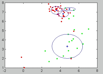
After preprocessing is found and applied on the data set, the experts training begins. Each expert has different number of cluster centers, and, optionally, different radii scales. The clusterings are found by the preprocessing procedure, and random choise of initial cluster centers in the k-means function contributes to experts independence. In addition, using different number of RBF centers will result in experts (with few centers), which can capture global patterns in the data, and others (with more centers) which are good in classifying local features. Their fusion will hopefully bring to better overall classification.

The number of experts and the number of hidden units in each expert is defined by a configuration parameter, if the parameter is not specified then a default set of number of hidden units which we found to be optimal is selected.

Each expert consists of an ensemble of networks with same architecture (same RBF clusters and radii). Each network is trained on the replicated fraction of the training set using bootstrapping technique with noise injection. Signals, which don't participate in training are used for cross-validation accross the ensemble. Each signal is thus used to validate different subset of ensemble members, and the scores are combined to give overall mean square error. As soon as the cross-validation error stops decreasing, the construction of ensemble stops. Thus best number of networks in the ensemble is determined on-line, from training results.

Related Files:

findarch.m

This is the main file which uses findpreproc to apply the preprocessing on the dataset and then creates all the experts. Experts are chosen with different number of centers, and k-means clustering is done for all of them, as described above. Each expert is then trained in turn by calling the train_expert function. The whole commitee of experts is stored in Matlab structure, which contains an commitee parameters, and array of structures describing each ensemble.

The train_expert function constructs the ensemble by creating different training sets for each new network. The set is generated by randomly putting data vectors to the sample, until the sample is of the same size as the data. This results in a sample, which contains about 63% of the data with replications. Gaussian noise is then added to the sample to prevent linear dependance, and RBF training procedure with BCM constraint is invoked. The procedure stops when cross-validation error stops decreasing, as explained above.

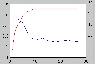
Using several networks in ensemble improves generalization ability of the expert by reducing variance component of the cross-validation error. However, too many networks in the ensemble may result in overfitting, and too large descriptor complexity. The above on-line procedure is meant to prevent this from happening. According to our tests, this procedure is indeed useful in creating good ensemble. The following figure depicts typical behaviour of the cross-validation error (blue), and number of signals, which participate in evaluation (red), as a function of the number of networks trained:

After the ensemble is created, a weight vector is generated according to the rank of each network in the ensemble in order to make "better" network in the ensemble influence more on the final prediction.

Outline of the network ensemble training algorithm:

1. First generate a new dataset which is a subset of the original data set using bootstraping technique (replication).
2. Add random noise to the newly created dataset in order to make all the networks as independent as possible.
3. Train a pair of networks, one predicting the reuqired output and one predicting the inverted output, using both networks in order to predict the output will make the prediction better. The training is done by a function that is passed as a parameter.
4. Save both networks in the return structure.
5. Create (analytically) the matrix that will be used for reconstruction of the input (used for confidence), and save that matrix too.
6. Calculate the error of the network on prediction of the test set (all the input vector that were not selected to the trainig set), and cross-validation error among the current ensemble, described above.
7. Repeat this until enough networks were created.

Rank ensemble will calculate the covariance matrix of the errors from all the networks in the ensemble, and use that to generate the weight vector.

The actual training is done by using the rbf_bcm function, however other functions can be given through the configuration structure.

The training is done using BCM constraint as an additional regularization parameter on the weight vector, it is implemented using gradient descent on both the BCM risk and the SSE. The regularization helps prevent overfitting of the network by introducing bias.

BCM projection index is applied to the network outputs, i.e. the network weights will define projections of the RBF activation values to direction of multimodality. This is done by calculating gradient vector, which minimizes BCM risk function E[x^3]/3 - E[x^2]^2/4 This risk function is then added as a regularization parameter to the learning error. This mixture of unsupervised and supervised learning will hopefully improve network generalization ability. in the space of RBF

On top of this a best regularization parameter on the weight vecotr (penalizing heavy weights) is found (by a simple test on all optional parameters).

Outline of the algorithm:

1. Start with initial weight vectors using the analytical solution (without any regularization parameter), and add a little noise in order to make the networks even more independent (change the starting point).
2. Calculate the gradient of the SSE and of the BCM risk with respect to the weight vector, make sure that both of the gradients have the same scale (we normalize the BCM gradient), in order to make sure that non of them will be dominant, both of the gradients should have the same effect.
3. Use gradient descent in order to update the weight vectors in a way that will minimize the error, the error is defined to be the sum of the SSE and the BCM risk.
   The learning rate changes dynamically, every iteration that succeeds in obtaining a smaller error value increases the learning rate, but once the error value increases, the weight are NOT updated and the learning rate is reduced in half, until the resulting gradient vector does decreases the error once more. This method helps the function converge much faster.
4. Continue the operation until the rate decreases to 0 (eps), or until too many iterations were performed.

rbf_bcm2.m

There is something wrong with this version, but it should be much better than the first one, in addition to what rbf_bcm is doing, here the gradient descent is also performed on the RBF centers and radiuses in order to find optimal values for the RBF representation, it uses the function CalcBCM in order to calculate the derivatives of the BCM risk with respect to the RBFs centers and radiuses.

This is not used!!!

CalcBCM.m

This is only used by rbf_bcm2.m (which is not used in the project because of some bug we couldn't find), it calculates the derivatives of the BCM risk for a given data set with respect to given centers and radiuses.

3. Using the network in order to predict new data

The function netpred will use an architecture and a preprocessing methodology found with findarch in order to predict the output of a new data set, it will also generate confidence values for the prediction according to the requested confidence type specified by a configuration parameter.

The prediction could be done either by a simple avaraging of all the networks in all the experts or by using the weights calculated by train_expert in order to change the influence of individual networks.

This will simply execute the preprocessing methodology saved in the preproc structure and then use the experts in the netarch structure to predict the output of the data set.

Several types of confidence are available:

1. Reconstruction - Try to reconstruct the input vectors using the matrix created while training the network, the value of the confidence of each network is the distance between the reconstructed vector and the original input vector.
2. Variance - Calculate the variance of the prediction value from ALL the networks (using weights if requested).
3. Value - Returned the non-boolean avarage value of the prediction across all networks (again, use weights if requested), the closer the value is to 0 the worse the prediction is.

Related Files:

netpred.m

Test results

We have also tested our k-means clustering algorithm, and have written the dataplot procedure for its visualization. The figure below depicts projection of the data and the clusters to 2-dimensional space of two most significant eigenvalues:

Using the functions

It is possible to use the functions without any configuration parameters, in which case a the default (optimal ?) values will be used, in order to change the default values, configuration parameters should be added according to the structure described in every functions help screen. In order for the functions to work, Orr's RBF toolbox, and Matlab statistics toolbox must be installed in Matlab's path.

The following is the syntax of main functions in the project:

[arch, preproc] = findarch(training_set, class_labels [,options]);

will create the architecture and preprocessing.

[processed, preproc] = findpreproc(training_set, class_labels, options [, preproc ])

will find preprocessing methodology for the data, or pass data through existing methodology. And

[pred, conf] = netpred(data_set, preproc, arch [,options]);

will generate the prediction and the confidence values. In additiom, k-means clustering can be obtained by:

[centers, radii] = mykmeans(max_clusters, data [, termination_error [, min_points_in_cluster] ])

and visualized by:

dataplot(data, labels, x, y [,centers [,radii [, colorscheme ]]]);

Remarks

We have quite a lot of ideas which we are still working on, including use of cross-validation to find best subset of experts, as well as some more test runs.

There is still a problem with the variant of RBF training with BCM algorithm, which would optimize centers and radii, as well as the weights, which we are still working on as well.