Project By:

Project Specifications:

• Preprocessing: Minimal entropy and clustering.
• Training constraints: BCM and Kurtosis.
• Architecture and code: Back-prop with LM.
• Confidence: Variance and your choice.
• Data: Sono and wvlet.

Project Overview:

A.  Preprocessing

1.  K-Means Clustering

- kmeans.m

This is the core function, receiving expected number of cluster (reduced dimension), data set, and several other parameters for running (like required iteration accuracy, max number of iterations, etc.), and returns the found K cluster centers for the data. It also provides some enhanced features, like auto reducing of "unjustified" cluster centers (i.e. centers that are too close to other centers in a way that does not "justify" their existence).

- prockmeans.m

This is the wrapper function, receiving data set and required dimension (optionally also previously found preprocessing parameters), then utilizing kmeans.m to find preprocessing (cluster centers) of given dimension. Next, it will process the data according to found (or given) preprocessing, and return it.

The outlines of the K-means clustering algorithm:

1. Guess some K cluster centers, for first iteration
2. Attach each data vector to the nearest (MSE) center.
3. Refine the cluster center to be the average of its vectors.
4. Remove empty clusters, if any, and re-guess new centers instead.
5. (Optional: reduce unjustified clusters)
6. If new (refined) centers differ from previous iteration, repeat from step (2).

Note that step (4) and (5) are additional to the original algorithm of K-means. Step (4) is considered elementary by us, since zero cluster centers are totally useless and meaning-less to the dimension reduction, and therefore are bound for replacing. Step (5), which is optional, is a little more complicated, and is done as follows:

• For each cluster, calculate "justification ratio" to be the minimal distance to other cluster centers divided by the mean of distances between cluster center and its vectors.
• For cluster with "smallest justification", if the distance to nearest cluster center goes below cluster inner mean distances * reduction factor (argument to the function), then reduce the cluster.

After calculation of the centers is accomplished, the new (reduced dimension) data is produced the following way: for each data vector, let the new coordination be the square of difference of each cluster center (respectively) normalized by the variance of this cluster (shifted by some constant epsilon, to avoid normalizing by zero).

Another improvement to the K-means cluster discovery, done by the wrapper function, is first finding K*log(K) cluster centers, then finding K cluster centers out of those K*log(K) intermediate vectors.

Finally, the K-means preprocessing data can be stored and returned for later use the following way:

1. The discovered cluster centers.
2. The variance of each cluster (used for normalizing the distances).

2.  Minimal Entropy Dimension Reduction

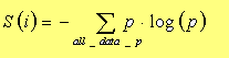
The entropy in each dimension is calculated in the usual way by the summation:

Where for every dimension the entropy is the summation of the multiplication of the data probabilistic density by its log. Since the data is not discrete the density function is made by calculating the histogram of the data set in each dimension. Another possible way for calculating the density (which has not been implemented), is by using instead of the usual square bins of the standard histogram, “Gaussian” bins. This could be made by passing it through a Gaussian filter that spreads out every data sample. In this way the density function calculated is smoother.

The minimal entropy dimension reduction is made by the following function:

- procminentropy.m

This function receives a data set and the dimension to which it should be reduced. If no such value is supplied then it leaves only the square root of the original dimensions. There is also an option of already entering the specific dimensions to be left, for later processing of vectors using previously found dimension reduction.
After calculating the entropy for each dimension, the function drops the dimensions with minimal entropy, thus leaving the dimensions with maximal entropy.
 

B.  Architecture Finding

Although finding the best dimension of the input is part of the preprocessing, the way we measure the quality of the chosen dimension is through the performance of the trained network (or ensemble of networks).

So both the decision about the dimension reduction (that also inflicts on the structure of the net) and the decision about the number of neurons in the hidden layer of the net are done in the light of the performance of the network.

As mentioned before we use an ensemble of networks for more stable and confident results.

The ensemble is constructed from 15 networks each trained on a subset of the data containing 80% from the samples, randomly chosen, in a way that a sample might be chosen more than once.

For each network we create a test subset that is the compliment of the training subset, on which the network will be checked.

We will know look how we find the best number of input and hidden neurons in practice:

In an external loop we iterate over the possible input dimensions starting from half the number of samples in the set (we could start from the number of the sample set, but we reduce it for performance) down to the square root of the number of samples.

The upper bound is because if we had more dimensions than samples we could use simple clustering for dimension reduction defining each input vector as a cluster center.

On the other hand we don't want to reduce the number of input dimension too much, because we might loose valuable information. We know that best training is done when the number of weights in the network is close to the number of input samples so reducing the input dimension below the square root of samples will not help us on the training while harm us in the loss of information.

For each combination of these numbers we calculate the average MSE of all networks in the ensemble and put it in a matrix.

After filling up the matrix, we find the minimal value of the matrix and the indexes of this value are the best-input and hidden layer dimensions for the ensemble.

The architecture finding is done using the findarch.m function.
 

C.  Confidence

1. Dynamic confidence that is different for each input given to the trained net, which is the variance of answer given by the ensemble. This confidence is calculated in netpred.m.
2. Static confidence that is constant for the trained network and is the average MSE, witthe ensemble, of the testing of each non the samples that it was not trained on. This type of confidence is calculated during training in findarch.m.

How to Run:

• options.preproc_options.method = ‘minimal entropy’ or ‘k-mean clustering’ preprocessing methods.
• options.net_options.method = ‘bcm’ or ‘kurtosis’ learning rule.
• options.conf_options = ‘variance’ or ‘bp’ for the fixed confidence.

Project Files: