Next: Solving the Unique Mapping
Up: DNA Physical Mapping
Previous: Unique Probe Mapping
PQ-Tree Algorithm [#!BL76!#]
A PQ-Tree is a rooted, ordered tree. We will use a PQ-tree
with the elements of U as leaves, and internal nodes of two
types: P-nodes and Q-nodes.
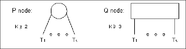
A P-node whose sub-nodes are
 for
for  represents k subsets of U (the leaf sets of
), each of which is known to be a consecutive
block of elements, but with the order of the blocks unknown. A
Q-node whose sub-nodes are
for
represents k subsets of U (the leaf sets of
), each of which is known to be a consecutive
block of elements, but with the order of the blocks unknown. A
Q-node whose sub-nodes are
for  represents that the k blocks corresponding to the leaf set of
are known to appear in this order, up to a
complete reversal (see figure 10.3).
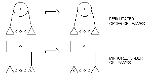
It is therefore clear that in order to have these meanings of the
P-nodes and Q-nodes we must allow the following legal
transformations (see figure 10.5
1 - 2).
represents that the k blocks corresponding to the leaf set of
are known to appear in this order, up to a
complete reversal (see figure 10.3).
It is therefore clear that in order to have these meanings of the
P-nodes and Q-nodes we must allow the following legal
transformations (see figure 10.5
1 - 2).
- 1.
- Reordering the sub-nodes of some P-node arbitrarily
- 2.
- Reversing the order of the sub-nodes of some Q-node

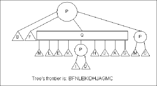
is the set
of all leaves, read in a left-to-right order. As demonstrated in
figure 10.4
Figure 10.3:
PQ-tree node types: we
use circles and bars to denote P-nodes and Q-nodes, respectively.
|
|
Figure 10.4:
Frontier of a PQ-tree
|
|
Figure 10.5:
Permitted
transformations of a PQ-tree
|
|
Figure 10.6:
Permitted
transformations of a PQ-tree
|
|
if there exists a set of legal transformations
leading from one tree to the other. In such a case, we write
 .
.

Therefore, the problem of permuting the probes in order to achieve
the consecutive 1's property of the STS matrix is equivalent to
finding a PQ-tree representing
 .
.
PQ-Tree Algorithm for Unique Probe DNA Mapping:
- 1.
- Initialize the tree as a root P-node with all elements of U as sub-nodes
(leaves).
- 2.
- For
 : reduce (T,Si)
The procedure reduce (T,Si) returns a tree for any
permutation in
consistent(T) in which Si is continuous.
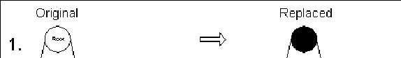
Reduce(T,Si)
- 1.
- Color all Si leaves.
- 2.
- Apply transformations to replace T with an equivalent
PQ-tree along whose frontier all of the colored leaves are
consecutive.
- 3.
- Identify the deepest node
Root(T,Si) whose subtree
spans all colored leaves
- 4.
- Apply replacement rules presented in figure 10.6 on this subtree, working
bottom-up till reaching
Root(T,Si)
Figure 10.7:
Example of PQ-tree
based algorithm
|
|
Figure 10.7 shows an example of application
of the PQ-Tree algorithm for unique probe DNA mapping.
The problem with using PQ-trees for solving the unique mapping
problem is that the algorithm does not support noise:
Unfortunately due to "real life" measurement errors the input
matrix usually has either extra or missing 1's entries. In such
case, the resulting PQ-tree10.1 will not produce the best
(minimum error) solution available, but rather an arbitrary
solution depending on the clone order chosen. Since all data is
obtained by experiments and errors are not uncommon, this
deficiency deters one from using the algorithm.
Next: Solving the Unique Mapping
Up: DNA Physical Mapping
Previous: Unique Probe Mapping
Itshack Pe`er
1999-03-21