Computing local alignment

Given a pair of indices ${i \leq n}$ and ${j \leq m}$ , the local suffix alignment problem is finding a (possibly empty) suffix ${\alpha}$ of $S_{1 \dots i}$ and a (possibly empty) suffix ${\beta}$ of $T_{1 \ldots j}$ such that the value of their alignment is the maximum over all values of alignments of suffixes of $S_{1 \ldots i}$ and $T_{1 \ldots j}$. We use V(i, j) to denote the value of the optimal local suffix alignment for a given pair i, j of indices.

We choose the weights of the editing operations as:

$${\sigma_(x,y)} = \left\{\begin{array}{ll} \ge 0 & \mbox{if $... ...f $x,y$ do not match or one of them is -} \end{array} \right.$$

The algorithm needs to:

1.

Find maximum similarity between suffixes of $S_{1 \ldots i}$ and $T_{1 \ldots j}$.

2.

Discard the prefixes $S_{1 \ldots i}, T_{1 \ldots j}$ whose similarity is $\le$ 0, and therfore decreases the overall similarity.

3.

Find the best indices i^*, j^* of S and T respectively after which the similarity only decreases.

Note that any extension of the optimal solution either to the right of to the left decreases the overall similarity.

Recursive definition: The base condition will be: V(i, 0) = 0 and 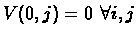${V(0, j) = 0 \ \forall i, j}$ since we can always choose an empty suffix.

For i > 0 and j > 0 the proper recurrence for V(i, j)is

$$V(i, j) = \max\{0, V(i - 1,j - 1) + \sigma_{(S_{i}, T_{j})}, ... ... 1) + \sigma_{(-, T_{j})}, V(i - 1, j) + \sigma_{(S_{i}, -)} \}$$

Compute i^*, j^* so that:

$${V(i^{*}, j^{*}) = \max_{1 \leq i \leq n, 1 \leq j \leq m} V(i, j)}$$

Observe that the recurrence for computing local suffix alignment is almost identical to the one used for computing global alignment. The only difference is the inclusion of zero in the case of local suffix alignment. In both global alignment and local suffix alignment of prefixes $S_{1 \ldots i}$ and $T_{1 \ldots j}$, the terminating characters of any alignment are specified, but in the case of local suffix alignment, any number of initial characters can be ignored.

The zero in the recurrence implements this, 'restarting' the recurrence. Adding 0 to the maximization makes sure that negative prefixes are discarded from the computation.

Adding the '0' to the constraint only handles mismatched prefixes, there's still a need to determine, when should a computation of a transformation be stopped, so that the similarity value will not decrease. Therefore, after computing the table of V(i, j) values, and there's a need to search for a cell with the maximal value and ignore all table entries from that point on.

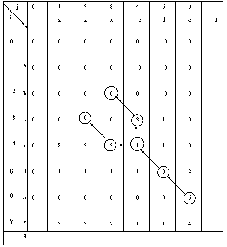
Example 2.14   Figure 2.3 illustrates the calculation of the $n\times{m}$ entries table for the two strings taken $\sigma$ as 2 for match and -1 for mismatch.

  

Figure 2.3: finding local alignment

As usual, pointers are created while filling in the values of the table. After cell (i^*, j*) is found, the substrings ${\alpha}$ and ${\beta}$ giving the optimal local alignment of S and T are found by tracing back the pointers from cell (i^*, j*) until reaching an entry (i', j') that has value zero. Then the optimal local alignment substrings are ${\alpha = S_{i' \ldots i^*}}$ and ${\beta = T_{j' \ldots j^*}}$. As it seems from here, space complexity will be O(mn), we will show that only O(m) space is needed:

Lemma 2.15   The optimal local alignment of two strings S and T can be computed in linear space.

Proof:The optimal local alignment of S and T identifies substrings ${\alpha}$ and ${\beta}$whose global alignment has maximum value over all pairs of substrings. Hence, if ${\alpha}$ and ${\beta}$ can be found using only linear space, then their actual alignment can be found in linear space, using Hirschberg's method for global alignment. The value of the optimal local alignment is found in cell i^*, j^*. Those indices specify the terminating points of the strings ${\alpha}$ and ${\beta}$. The values of each row can be computed in a row wise fasion and the algorithm must store values for only two rows at a time. Hence, the end positions (i^*, j^*) can be computed in linear space. To find the starting position of the two substrings, the algorithm can execute the reverse dynamic programing using linear space (the details are left as an exercise).

Complexity :

• Time Complexity - since it takes constant number of operation per cell to compute V(i, j), it takes only O(mn) time to fill in the entire table. The search for V(i*, j*) requires only O(nm) time as well. Hence the total time complexity is O(nm).

• Space Complexity - As shown in lemma local alignment, the space complexity is O(m).